Recent Tutorials
Introduction to Artificial Neural Networks - Part 1
This is the first part of a three part introductory tutorial on artificial neural networks. In this first tutorial we will discover what neural networks are, why they’re useful for solving certain types of tasks and finally how they work.
Introduction
Computers are great at solving algorithmic and math problems, but often the world can’t easily be defined with a mathematical algorithm. Facial recognition and language processing are a couple of examples of problems that can’t easily be quantified into an algorithm, however these tasks are trivial to humans. The key to Artificial Neural Networks is that their design enables them to process information in a similar way to our own biological brains, by drawing inspiration from how our own nervous system functions. This makes them useful tools for solving problems like facial recognition, which our biological brains can do easily.How do they work?
First lets take a look at what a biological neuron looks like.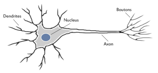
Our brains use extremely large interconnected networks of neurons to process information and model the world we live in. Electrical inputs are passed through this network of neurons which result in an output being produced. In the case of a biological brain this could result in contracting a muscle or signaling your sweat glands to produce sweat. A neuron collects inputs using a structure called dendrites, the neuron effectively sums all of these inputs from the dendrites and if the resulting value is greater than it’s firing threshold, the neuron fires. When the neuron fires it sends an electrical impulse through the neuron’s axon to it’s boutons. These boutons can then be networked to thousands of other neurons via connections called synapses. There are about one hundred billion (100,000,000,000) neurons inside the human brain each with about one thousand synaptic connections. It’s effectively the way in which these synapses are wired that give our brains the ability to process information the way they do.
Modeling Artificial Neurons
Artificial neuron models are at their core simplified models based on biological neurons. This allows them to capture the essence of how a biological neuron functions. We usually refer to these artificial neurons as ‘perceptrons’. So now lets take a look at what a perceptron looks like.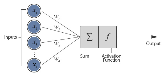
As shown in the diagram above a typical perceptron will have many inputs and these inputs are all individually weighted. The perceptron weights can either amplify or deamplify the original input signal. For example, if the input is 1 and the input’s weight is 0.2 the input will be decreased to 0.2. These weighted signals are then added together and passed into the activation function. The activation function is used to convert the input into a more useful output. There are many different types of activation function but one of the simplest would be step function. A step function will typically output a 1 if the input is higher than a certain threshold, otherwise it’s output will be 0.
Here’s an example of how this might work:
Input 2 (x2) = 1.0
Weight 1 (w1) = 0.5
Weight 2 (w2) = 0.8
Threshold = 1.0
First we multiple the inputs by their weights and sum them:
Now we compare our input total to the perceptron’s activation threshold. In this example the total input (1.1) is higher than the activation threshold (1.0) so the neuron would fire.
Implementing Artificial Neural Networks
So now you’re probably wondering what an artificial neural network looks like and how it uses these artificial neurons to process information. In this tutorial we’re going to be looking at feedforward networks and how their design links our perceptron together creating a functioning artificial neural network. Before we begin lets take a look at what a basic feedforward network looks like: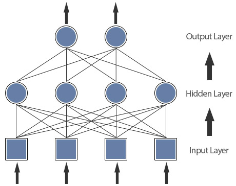
Each input from the input layer is fed up to each node in the hidden layer, and from there to each node on the output layer. We should note that there can be any number of nodes per layer and there are usually multiple hidden layers to pass through before ultimately reaching the output layer. Choosing the right number of nodes and layers is important later on when optimising the neural network to work well a given problem. As you can probably tell from the diagram, it’s called a feedforward network because of how the signals are passed through the layers of the neural network in a single direction. These aren’t the only type of neural network though. There are also feedback networks where its architecture allows signals to travel in both directions.
Linear separability
To explain why we usually require a hidden layer to solve our problem, take a look at the following examples:
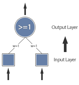
Notice how the OR function can be separated on the graph with a single straight line, this means the function is “linearly separable” and can be modelled within our neural network without implementing a hidden layer, for example, the OR function can be modeled with a single perceptron like this:
However to model the XOR function we need to use an extra layer:
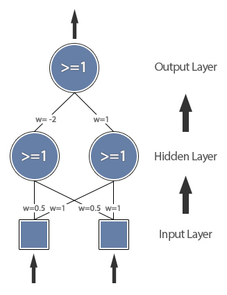
We call this type of neural network a ‘multi layer perceptron’. In almost every case you should only ever need to use one or two hidden layers, however it make take more experimentation to find the optimal amount of nodes for the hidden layer(s).
To be continued...
So now you should have a basic understanding of some of the typical applications for neural networks and why we use them for these purposes. You should also have a rough understanding of how a basic neural network operates and how it can process data. In the next tutorial we will be looking at ways to construct a neural network and then how we can ‘train’ it to do the things we want it to do.Part 2 is now available here, Introduction to Artificial Neural Networks Part 2 - Learning
Simulated Annealing for beginners
Finding an optimal solution for certain optimisation problems can be an incredibly difficult task, often practically impossible. This is because when a problem gets sufficiently large we need to search through an enormous number of possible solutions to find the optimal one. Even with modern computing power there are still often too many possible solutions to consider. In this case because we can’t realistically expect to find the optimal one within a sensible length of time, we have to settle for something that’s close enough.
An example optimisation problem which usually has a large number of possible solutions would be the traveling salesman problem. In order to find a solution to a problem such as the traveling salesman problem we need to use an algorithm that’s able to find a good enough solution in a reasonable amount of time. In a previous tutorial we looked at how we could do this with genetic algorithms, and although genetic algorithms are one way we can find a ‘good-enough’ solution to the traveling salesman problem, there are other simpler algorithms we can implement that will also find us a close to optimal solution. In this tutorial the algorithm we will be using is, ‘simulated annealing’.
If you’re not familiar with the traveling salesman problem it might be worth taking a look at my previous tutorial before continuing.
What is Simulated Annealing?
First, let’s look at how simulated annealing works, and why it’s good at finding solutions to the traveling salesman problem in particular. The simulated annealing algorithm was originally inspired from the process of annealing in metal work. Annealing involves heating and cooling a material to alter its physical properties due to the changes in its internal structure. As the metal cools its new structure becomes fixed, consequently causing the metal to retain its newly obtained properties. In simulated annealing we keep a temperature variable to simulate this heating process. We initially set it high and then allow it to slowly ‘cool’ as the algorithm runs. While this temperature variable is high the algorithm will be allowed, with more frequency, to accept solutions that are worse than our current solution. This gives the algorithm the ability to jump out of any local optimums it finds itself in early on in execution. As the temperature is reduced so is the chance of accepting worse solutions, therefore allowing the algorithm to gradually focus in on a area of the search space in which hopefully, a close to optimum solution can be found. This gradual ‘cooling’ process is what makes the simulated annealing algorithm remarkably effective at finding a close to optimum solution when dealing with large problems which contain numerous local optimums. The nature of the traveling salesman problem makes it a perfect example.Advantages of Simulated Annealing
You may be wondering if there is any real advantage to implementing simulated annealing over something like a simple hill climber. Although hill climbers can be surprisingly effective at finding a good solution, they also have a tendency to get stuck in local optimums. As we previously determined, the simulated annealing algorithm is excellent at avoiding this problem and is much better on average at finding an approximate global optimum.To help better understand let’s quickly take a look at why a basic hill climbing algorithm is so prone to getting caught in local optimums.
A hill climber algorithm will simply accept neighbour solutions that are better than the current solution. When the hill climber can’t find any better neighbours, it stops.
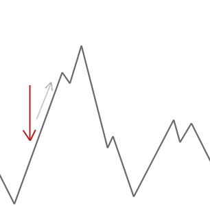
In the example above we start our hill climber off at the red arrow and it works its way up the hill until it reaches a point where it can’t climb any higher without first descending. In this example we can clearly see that it’s stuck in a local optimum. If this were a real world problem we wouldn’t know how the search space looks so unfortunately we wouldn’t be able to tell whether this solution is anywhere close to a global optimum.
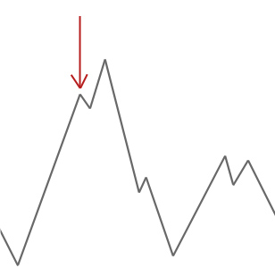
Simulated annealing works slightly differently than this and will occasionally accept worse solutions. This characteristic of simulated annealing helps it to jump out of any local optimums it might have otherwise got stuck in.
Acceptance Function
Let’s take a look at how the algorithm decides which solutions to accept so we can better understand how its able to avoid these local optimums.First we check if the neighbour solution is better than our current solution. If it is, we accept it unconditionally. If however, the neighbour solution isn’t better we need to consider a couple of factors. Firstly, how much worse the neighbour solution is; and secondly, how high the current ‘temperature’ of our system is. At high temperatures the system is more likely accept solutions that are worse.
The math for this is pretty simple:
Basically, the smaller the change in energy (the quality of the solution), and the higher the temperature, the more likely it is for the algorithm to accept the solution.
Algorithm Overview
So how does the algorithm look? Well, in its most basic implementation it’s pretty simple.- First we need set the initial temperature and create a random initial solution.
- Then we begin looping until our stop condition is met. Usually either the system has sufficiently cooled, or a good-enough solution has been found.
- From here we select a neighbour by making a small change to our current solution.
- We then decide whether to move to that neighbour solution.
- Finally, we decrease the temperature and continue looping
Temperature Initialisation
For better optimisation, when initialising the temperature variable we should select a temperature that will initially allow for practically any move against the current solution. This gives the algorithm the ability to better explore the entire search space before cooling and settling in a more focused region.Example Code
Now let’s use what we know to create a basic simulated annealing algorithm, and then apply it to the traveling salesman problem below. We’re going to use Java in this tutorial, but the logic should hopefully be simple enough to copy to any language of your choice.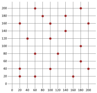
First we need to create a City class that can be used to model the different destinations of our traveling salesman.
City.java
* City.java
* Models a city
*/
package sa;
public class City {
int x;
int y;
// Constructs a randomly placed city
public City(){
this.x = (int)(Math.random()*200);
this.y = (int)(Math.random()*200);
}
// Constructs a city at chosen x, y location
public City(int x, int y){
this.x = x;
this.y = y;
}
// Gets city's x coordinate
public int getX(){
return this.x;
}
// Gets city's y coordinate
public int getY(){
return this.y;
}
// Gets the distance to given city
public double distanceTo(City city){
int xDistance = Math.abs(getX() - city.getX());
int yDistance = Math.abs(getY() - city.getY());
double distance = Math.sqrt( (xDistance*xDistance) + (yDistance*yDistance) );
return distance;
}
@Override
public String toString(){
return getX()+", "+getY();
}
}
Next let’s create a class that can keep track of the cities.
TourManager.java
* TourManager.java
* Holds the cities of a tour
*/
package sa;
import java.util.ArrayList;
public class TourManager {
// Holds our cities
private static ArrayList destinationCities = new ArrayList<City>();
// Adds a destination city
public static void addCity(City city) {
destinationCities.add(city);
}
// Get a city
public static City getCity(int index){
return (City)destinationCities.get(index);
}
// Get the number of destination cities
public static int numberOfCities(){
return destinationCities.size();
}
}
Now to create the class that can model a traveling salesman tour.
Tour.java
* Tour.java
* Stores a candidate tour through all cities
*/
package sa;
import java.util.ArrayList;
import java.util.Collections;
public class Tour{
// Holds our tour of cities
private ArrayList tour = new ArrayList<City>();
// Cache
private int distance = 0;
// Constructs a blank tour
public Tour(){
for (int i = 0; i < TourManager.numberOfCities(); i++) {
tour.add(null);
}
}
// Constructs a tour from another tour
public Tour(ArrayList tour){
this.tour = (ArrayList) tour.clone();
}
// Returns tour information
public ArrayList getTour(){
return tour;
}
// Creates a random individual
public void generateIndividual() {
// Loop through all our destination cities and add them to our tour
for (int cityIndex = 0; cityIndex < TourManager.numberOfCities(); cityIndex++) {
setCity(cityIndex, TourManager.getCity(cityIndex));
}
// Randomly reorder the tour
Collections.shuffle(tour);
}
// Gets a city from the tour
public City getCity(int tourPosition) {
return (City)tour.get(tourPosition);
}
// Sets a city in a certain position within a tour
public void setCity(int tourPosition, City city) {
tour.set(tourPosition, city);
// If the tours been altered we need to reset the fitness and distance
distance = 0;
}
// Gets the total distance of the tour
public int getDistance(){
if (distance == 0) {
int tourDistance = 0;
// Loop through our tour's cities
for (int cityIndex=0; cityIndex < tourSize(); cityIndex++) {
// Get city we're traveling from
City fromCity = getCity(cityIndex);
// City we're traveling to
City destinationCity;
// Check we're not on our tour's last city, if we are set our
// tour's final destination city to our starting city
if(cityIndex+1 < tourSize()){
destinationCity = getCity(cityIndex+1);
}
else{
destinationCity = getCity(0);
}
// Get the distance between the two cities
tourDistance += fromCity.distanceTo(destinationCity);
}
distance = tourDistance;
}
return distance;
}
// Get number of cities on our tour
public int tourSize() {
return tour.size();
}
@Override
public String toString() {
String geneString = "|";
for (int i = 0; i < tourSize(); i++) {
geneString += getCity(i)+"|";
}
return geneString;
}
}
Finally, let’s create our simulated annealing algorithm.
SimulatedAnnealing.java
public class SimulatedAnnealing {
// Calculate the acceptance probability
public static double acceptanceProbability(int energy, int newEnergy, double temperature) {
// If the new solution is better, accept it
if (newEnergy < energy) {
return 1.0;
}
// If the new solution is worse, calculate an acceptance probability
return Math.exp((energy - newEnergy) / temperature);
}
public static void main(String[] args) {
// Create and add our cities
City city = new City(60, 200);
TourManager.addCity(city);
City city2 = new City(180, 200);
TourManager.addCity(city2);
City city3 = new City(80, 180);
TourManager.addCity(city3);
City city4 = new City(140, 180);
TourManager.addCity(city4);
City city5 = new City(20, 160);
TourManager.addCity(city5);
City city6 = new City(100, 160);
TourManager.addCity(city6);
City city7 = new City(200, 160);
TourManager.addCity(city7);
City city8 = new City(140, 140);
TourManager.addCity(city8);
City city9 = new City(40, 120);
TourManager.addCity(city9);
City city10 = new City(100, 120);
TourManager.addCity(city10);
City city11 = new City(180, 100);
TourManager.addCity(city11);
City city12 = new City(60, 80);
TourManager.addCity(city12);
City city13 = new City(120, 80);
TourManager.addCity(city13);
City city14 = new City(180, 60);
TourManager.addCity(city14);
City city15 = new City(20, 40);
TourManager.addCity(city15);
City city16 = new City(100, 40);
TourManager.addCity(city16);
City city17 = new City(200, 40);
TourManager.addCity(city17);
City city18 = new City(20, 20);
TourManager.addCity(city18);
City city19 = new City(60, 20);
TourManager.addCity(city19);
City city20 = new City(160, 20);
TourManager.addCity(city20);
// Set initial temp
double temp = 10000;
// Cooling rate
double coolingRate = 0.003;
// Initialize intial solution
Tour currentSolution = new Tour();
currentSolution.generateIndividual();
System.out.println("Initial solution distance: " + currentSolution.getDistance());
// Set as current best
Tour best = new Tour(currentSolution.getTour());
// Loop until system has cooled
while (temp > 1) {
// Create new neighbour tour
Tour newSolution = new Tour(currentSolution.getTour());
// Get a random positions in the tour
int tourPos1 = (int) (newSolution.tourSize() * Math.random());
int tourPos2 = (int) (newSolution.tourSize() * Math.random());
// Get the cities at selected positions in the tour
City citySwap1 = newSolution.getCity(tourPos1);
City citySwap2 = newSolution.getCity(tourPos2);
// Swap them
newSolution.setCity(tourPos2, citySwap1);
newSolution.setCity(tourPos1, citySwap2);
// Get energy of solutions
int currentEnergy = currentSolution.getDistance();
int neighbourEnergy = newSolution.getDistance();
// Decide if we should accept the neighbour
if (acceptanceProbability(currentEnergy, neighbourEnergy, temp) > Math.random()) {
currentSolution = new Tour(newSolution.getTour());
}
// Keep track of the best solution found
if (currentSolution.getDistance() < best.getDistance()) {
best = new Tour(currentSolution.getTour());
}
// Cool system
temp *= 1-coolingRate;
}
System.out.println("Final solution distance: " + best.getDistance());
System.out.println("Tour: " + best);
}
}
Output
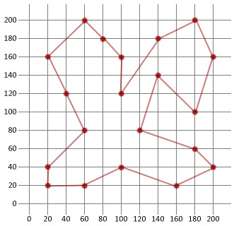
Final solution distance: 911
Tour: |180, 200|200, 160|140, 140|180, 100|180, 60|200, 40|160, 20|120, 80|100, 40|60, 20|20, 20|20, 40|60, 80|100, 120|40, 120|20, 160|60, 200|80, 180|100, 160|140, 180|
Conclusion
In this example we were able to more than half the distance of our initial randomly generated route. This hopefully goes to show how handy this relatively simple algorithm is when applied to certain types of optimisation problems.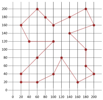
Applying a genetic algorithm to the traveling salesman problem
To understand what the traveling salesman problem (TSP) is, and why it's so problematic, let's briefly go over a classic example of the problem.
Imagine you're a salesman and you've been given a map like the one opposite. On it you see that the map contains a total of 20 locations and you're told it’s your job to visit each of these locations to make a sell.
Before you set off on your journey you'll probably want to plan a route so you can minimize your travel time. Fortunately, humans are pretty good at this, we can easily work out a reasonably good route without needing to do much more than glance at the map. However, when we’ve found a route that we believe is optimal, how can we test if it's really the optimal route?
Well, in short, we can’t - at least not practically.
To understand why it's so difficult to prove the optimal route let’s consider a similar map with just 3 locations instead of the original 20. To find a single route, we first have to choose a starting location from the three possible locations on the map. Next, we’d have a choice of 2 cities for the second location, then finally there is just 1 city left to pick to complete our route. This would mean there are 3 x 2 x 1 different routes to pick in total.
That means, for this example, there are only 6 different routes to pick from. So for this case of just 3 locations it's reasonably trivial to calculate each of those 6 routes and find the shortest. If you're good at maths you may have already realized what the problem is here. The number of possible routes is a factorial of the number of locations to visit, and trouble with factorials is that they grow in size remarkably quick!
For example, the factorial of 10 is 3628800, but the factorial of 20 is a gigantic, 2432902008176640000.
So going back to our original problem, if we want to find the shortest route for our map of 20 locations we would have to evaluate 2432902008176640000 different routes! Even with modern computing power this is terribly impractical, and for even bigger problems, it’s close to impossible.
Finding a solution
Although it may not be practical to find the best solution for a problem like ours, we do have algorithms that let us discover close to optimum solutions such as the nearest neighbor algorithm and swarm optimization. These algorithms are capable of finding a ‘good-enough’ solution to the travelling salesman problem surprisingly quickly. In this tutorial however, we will be using genetic algorithms as our optimization technique.If you’re not already familiar with genetic algorithms and like to know how they work, then please have a look at the introductory tutorial below:
Creating a genetic algorithm for beginners
Finding a solution to the travelling salesman problem requires we set up a genetic algorithm in a specialized way. For instance, a valid solution would need to represent a route where every location is included at least once and only once. If a route contain a single location more than once, or missed a location out completely it wouldn't be valid and we would be valuable computation time calculating it's distance.
To ensure the genetic algorithm does indeed meet this requirement special types of mutation and crossover methods are needed.
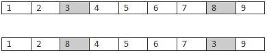
Firstly, the mutation method should only be capable of shuffling the route, it shouldn't ever add or remove a location from the route, otherwise it would risk creating an invalid solution. One type of mutation method we could use is swap mutation.
With swap mutation two location in the route are selected at random then their positions are simply swapped. For example, if we apply swap mutation to the following list, [1,2,3,4,5] we might end up with, [1,2,5,4,3]. Here, positions 3 and 5 were switched creating a new list with exactly the same values, just a different order. Because swap mutation is only swapping pre-existing values, it will never create a list which has missing or duplicate values when compared to the original, and that's exactly what we want for the traveling salesman problem.
Now we’ve dealt with the mutation method we need to pick a crossover method which can enforce the same constraint.
One crossover method that's able to produce a valid route is ordered crossover. In this crossover method we select a subset from the first parent, and then add that subset to the offspring. Any missing values are then adding to the offspring from the second parent in order that they are found.
To make this explanation a little clearer consider the following example:
Parents
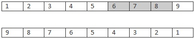
Offspring
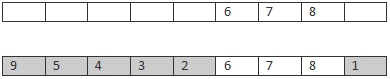
Here a subset of the route is taken from the first parent (6,7,8) and added to the offspring's route. Next, the missing route locations are adding in order from the second parent. The first location in the second parent's route is 9 which isn't in the offspring's route so it's added in the first available position. The next position in the parents route is 8 which is in the offspring's route so it's skipped. This process continues until the offspring has no remaining empty values. If implemented correctly the end result should be a route which contains all of the positions it's parents did with no positions missing or duplicated.
Creating the Genetic Algorithm
In literature of the traveling salesman problem since locations are typically refereed to as cities, and routes are refereed to as tours, we will adopt the standard naming conventions in our code.To start, let’s create a class that can encode the cities.
City.java
* City.java
* Models a city
*/
package tsp;
public class City {
int x;
int y;
// Constructs a randomly placed city
public City(){
this.x = (int)(Math.random()*200);
this.y = (int)(Math.random()*200);
}
// Constructs a city at chosen x, y location
public City(int x, int y){
this.x = x;
this.y = y;
}
// Gets city's x coordinate
public int getX(){
return this.x;
}
// Gets city's y coordinate
public int getY(){
return this.y;
}
// Gets the distance to given city
public double distanceTo(City city){
int xDistance = Math.abs(getX() - city.getX());
int yDistance = Math.abs(getY() - city.getY());
double distance = Math.sqrt( (xDistance*xDistance) + (yDistance*yDistance) );
return distance;
}
@Override
public String toString(){
return getX()+", "+getY();
}
}
Now we can create a class that holds all of our destination cities for our tour
TourManager.java
* TourManager.java
* Holds the cities of a tour
*/
package tsp;
import java.util.ArrayList;
public class TourManager {
// Holds our cities
private static ArrayList destinationCities = new ArrayList<City>();
// Adds a destination city
public static void addCity(City city) {
destinationCities.add(city);
}
// Get a city
public static City getCity(int index){
return (City)destinationCities.get(index);
}
// Get the number of destination cities
public static int numberOfCities(){
return destinationCities.size();
}
}
Next we need a class that can encode our routes, these are generally referred to as tours so we'll stick to the convention.
Tour.java
* Tour.java
* Stores a candidate tour
*/
package tsp;
import java.util.ArrayList;
import java.util.Collections;
public class Tour{
// Holds our tour of cities
private ArrayList tour = new ArrayList<City>();
// Cache
private double fitness = 0;
private int distance = 0;
// Constructs a blank tour
public Tour(){
for (int i = 0; i < TourManager.numberOfCities(); i++) {
tour.add(null);
}
}
public Tour(ArrayList tour){
this.tour = tour;
}
// Creates a random individual
public void generateIndividual() {
// Loop through all our destination cities and add them to our tour
for (int cityIndex = 0; cityIndex < TourManager.numberOfCities(); cityIndex++) {
setCity(cityIndex, TourManager.getCity(cityIndex));
}
// Randomly reorder the tour
Collections.shuffle(tour);
}
// Gets a city from the tour
public City getCity(int tourPosition) {
return (City)tour.get(tourPosition);
}
// Sets a city in a certain position within a tour
public void setCity(int tourPosition, City city) {
tour.set(tourPosition, city);
// If the tours been altered we need to reset the fitness and distance
fitness = 0;
distance = 0;
}
// Gets the tours fitness
public double getFitness() {
if (fitness == 0) {
fitness = 1/(double)getDistance();
}
return fitness;
}
// Gets the total distance of the tour
public int getDistance(){
if (distance == 0) {
int tourDistance = 0;
// Loop through our tour's cities
for (int cityIndex=0; cityIndex < tourSize(); cityIndex++) {
// Get city we're travelling from
City fromCity = getCity(cityIndex);
// City we're travelling to
City destinationCity;
// Check we're not on our tour's last city, if we are set our
// tour's final destination city to our starting city
if(cityIndex+1 < tourSize()){
destinationCity = getCity(cityIndex+1);
}
else{
destinationCity = getCity(0);
}
// Get the distance between the two cities
tourDistance += fromCity.distanceTo(destinationCity);
}
distance = tourDistance;
}
return distance;
}
// Get number of cities on our tour
public int tourSize() {
return tour.size();
}
// Check if the tour contains a city
public boolean containsCity(City city){
return tour.contains(city);
}
@Override
public String toString() {
String geneString = "|";
for (int i = 0; i < tourSize(); i++) {
geneString += getCity(i)+"|";
}
return geneString;
}
}
We also need to create a class that can hold a population of candidate tours
Population.java
* Population.java
* Manages a population of candidate tours
*/
package tsp;
public class Population {
// Holds population of tours
Tour[] tours;
// Construct a population
public Population(int populationSize, boolean initialise) {
tours = new Tour[populationSize];
// If we need to initialise a population of tours do so
if (initialise) {
// Loop and create individuals
for (int i = 0; i < populationSize(); i++) {
Tour newTour = new Tour();
newTour.generateIndividual();
saveTour(i, newTour);
}
}
}
// Saves a tour
public void saveTour(int index, Tour tour) {
tours[index] = tour;
}
// Gets a tour from population
public Tour getTour(int index) {
return tours[index];
}
// Gets the best tour in the population
public Tour getFittest() {
Tour fittest = tours[0];
// Loop through individuals to find fittest
for (int i = 1; i < populationSize(); i++) {
if (fittest.getFitness() <= getTour(i).getFitness()) {
fittest = getTour(i);
}
}
return fittest;
}
// Gets population size
public int populationSize() {
return tours.length;
}
}
Next, the let's create a GA class which will handle the working of the genetic algorithm and evolve our population of solutions.
GA.java
* GA.java
* Manages algorithms for evolving population
*/
package tsp;
public class GA {
/* GA parameters */
private static final double mutationRate = 0.015;
private static final int tournamentSize = 5;
private static final boolean elitism = true;
// Evolves a population over one generation
public static Population evolvePopulation(Population pop) {
Population newPopulation = new Population(pop.populationSize(), false);
// Keep our best individual if elitism is enabled
int elitismOffset = 0;
if (elitism) {
newPopulation.saveTour(0, pop.getFittest());
elitismOffset = 1;
}
// Crossover population
// Loop over the new population's size and create individuals from
// Current population
for (int i = elitismOffset; i < newPopulation.populationSize(); i++) {
// Select parents
Tour parent1 = tournamentSelection(pop);
Tour parent2 = tournamentSelection(pop);
// Crossover parents
Tour child = crossover(parent1, parent2);
// Add child to new population
newPopulation.saveTour(i, child);
}
// Mutate the new population a bit to add some new genetic material
for (int i = elitismOffset; i < newPopulation.populationSize(); i++) {
mutate(newPopulation.getTour(i));
}
return newPopulation;
}
// Applies crossover to a set of parents and creates offspring
public static Tour crossover(Tour parent1, Tour parent2) {
// Create new child tour
Tour child = new Tour();
// Get start and end sub tour positions for parent1's tour
int startPos = (int) (Math.random() * parent1.tourSize());
int endPos = (int) (Math.random() * parent1.tourSize());
// Loop and add the sub tour from parent1 to our child
for (int i = 0; i < child.tourSize(); i++) {
// If our start position is less than the end position
if (startPos < endPos && i > startPos && i < endPos) {
child.setCity(i, parent1.getCity(i));
} // If our start position is larger
else if (startPos > endPos) {
if (!(i < startPos && i > endPos)) {
child.setCity(i, parent1.getCity(i));
}
}
}
// Loop through parent2's city tour
for (int i = 0; i < parent2.tourSize(); i++) {
// If child doesn't have the city add it
if (!child.containsCity(parent2.getCity(i))) {
// Loop to find a spare position in the child's tour
for (int ii = 0; ii < child.tourSize(); ii++) {
// Spare position found, add city
if (child.getCity(ii) == null) {
child.setCity(ii, parent2.getCity(i));
break;
}
}
}
}
return child;
}
// Mutate a tour using swap mutation
private static void mutate(Tour tour) {
// Loop through tour cities
for(int tourPos1=0; tourPos1 < tour.tourSize(); tourPos1++){
// Apply mutation rate
if(Math.random() < mutationRate){
// Get a second random position in the tour
int tourPos2 = (int) (tour.tourSize() * Math.random());
// Get the cities at target position in tour
City city1 = tour.getCity(tourPos1);
City city2 = tour.getCity(tourPos2);
// Swap them around
tour.setCity(tourPos2, city1);
tour.setCity(tourPos1, city2);
}
}
}
// Selects candidate tour for crossover
private static Tour tournamentSelection(Population pop) {
// Create a tournament population
Population tournament = new Population(tournamentSize, false);
// For each place in the tournament get a random candidate tour and
// add it
for (int i = 0; i < tournamentSize; i++) {
int randomId = (int) (Math.random() * pop.populationSize());
tournament.saveTour(i, pop.getTour(randomId));
}
// Get the fittest tour
Tour fittest = tournament.getFittest();
return fittest;
}
}
Now we can create our main method, add our cities and evolve a route for our travelling salesman problem.
TSP_GA.java
* TSP_GA.java
* Create a tour and evolve a solution
*/
package tsp;
public class TSP_GA {
public static void main(String[] args) {
// Create and add our cities
City city = new City(60, 200);
TourManager.addCity(city);
City city2 = new City(180, 200);
TourManager.addCity(city2);
City city3 = new City(80, 180);
TourManager.addCity(city3);
City city4 = new City(140, 180);
TourManager.addCity(city4);
City city5 = new City(20, 160);
TourManager.addCity(city5);
City city6 = new City(100, 160);
TourManager.addCity(city6);
City city7 = new City(200, 160);
TourManager.addCity(city7);
City city8 = new City(140, 140);
TourManager.addCity(city8);
City city9 = new City(40, 120);
TourManager.addCity(city9);
City city10 = new City(100, 120);
TourManager.addCity(city10);
City city11 = new City(180, 100);
TourManager.addCity(city11);
City city12 = new City(60, 80);
TourManager.addCity(city12);
City city13 = new City(120, 80);
TourManager.addCity(city13);
City city14 = new City(180, 60);
TourManager.addCity(city14);
City city15 = new City(20, 40);
TourManager.addCity(city15);
City city16 = new City(100, 40);
TourManager.addCity(city16);
City city17 = new City(200, 40);
TourManager.addCity(city17);
City city18 = new City(20, 20);
TourManager.addCity(city18);
City city19 = new City(60, 20);
TourManager.addCity(city19);
City city20 = new City(160, 20);
TourManager.addCity(city20);
// Initialize population
Population pop = new Population(50, true);
System.out.println("Initial distance: " + pop.getFittest().getDistance());
// Evolve population for 100 generations
pop = GA.evolvePopulation(pop);
for (int i = 0; i < 100; i++) {
pop = GA.evolvePopulation(pop);
}
// Print final results
System.out.println("Finished");
System.out.println("Final distance: " + pop.getFittest().getDistance());
System.out.println("Solution:");
System.out.println(pop.getFittest());
}
}
Output:
Finished
Final distance: 940
Solution:
|60, 200|20, 160|40, 120|60, 80|20, 40|20, 20|60, 20|100, 40|160, 20|200, 40|180, 60|120, 80|140, 140|180, 100|200, 160|180, 200|140, 180|100, 120|100, 160|80, 180|
As you can see in just 100 generations we were able to find a route just over twice as good as our original and probably pretty close to optimum.
Final Results:
If you liked this tutorial you might also enjoy, Simulated Annealing for beginners