Simulated Annealing for beginners
Finding an optimal solution for certain optimisation problems can be an incredibly difficult task, often practically impossible. This is because when a problem gets sufficiently large we need to search through an enormous number of possible solutions to find the optimal one. Even with modern computing power there are still often too many possible solutions to consider. In this case because we can’t realistically expect to find the optimal one within a sensible length of time, we have to settle for something that’s close enough.An example optimisation problem which usually has a large number of possible solutions would be the traveling salesman problem. In order to find a solution to a problem such as the traveling salesman problem we need to use an algorithm that’s able to find a good enough solution in a reasonable amount of time. In a previous tutorial we looked at how we could do this with genetic algorithms, and although genetic algorithms are one way we can find a ‘good-enough’ solution to the traveling salesman problem, there are other simpler algorithms we can implement that will also find us a close to optimal solution. In this tutorial the algorithm we will be using is, ‘simulated annealing’.
If you’re not familiar with the traveling salesman problem it might be worth taking a look at my previous tutorial before continuing.
What is Simulated Annealing?
First, let’s look at how simulated annealing works, and why it’s good at finding solutions to the traveling salesman problem in particular. The simulated annealing algorithm was originally inspired from the process of annealing in metal work. Annealing involves heating and cooling a material to alter its physical properties due to the changes in its internal structure. As the metal cools its new structure becomes fixed, consequently causing the metal to retain its newly obtained properties. In simulated annealing we keep a temperature variable to simulate this heating process. We initially set it high and then allow it to slowly ‘cool’ as the algorithm runs. While this temperature variable is high the algorithm will be allowed, with more frequency, to accept solutions that are worse than our current solution. This gives the algorithm the ability to jump out of any local optimums it finds itself in early on in execution. As the temperature is reduced so is the chance of accepting worse solutions, therefore allowing the algorithm to gradually focus in on a area of the search space in which hopefully, a close to optimum solution can be found. This gradual ‘cooling’ process is what makes the simulated annealing algorithm remarkably effective at finding a close to optimum solution when dealing with large problems which contain numerous local optimums. The nature of the traveling salesman problem makes it a perfect example.Advantages of Simulated Annealing
You may be wondering if there is any real advantage to implementing simulated annealing over something like a simple hill climber. Although hill climbers can be surprisingly effective at finding a good solution, they also have a tendency to get stuck in local optimums. As we previously determined, the simulated annealing algorithm is excellent at avoiding this problem and is much better on average at finding an approximate global optimum.To help better understand let’s quickly take a look at why a basic hill climbing algorithm is so prone to getting caught in local optimums.
A hill climber algorithm will simply accept neighbour solutions that are better than the current solution. When the hill climber can’t find any better neighbours, it stops.
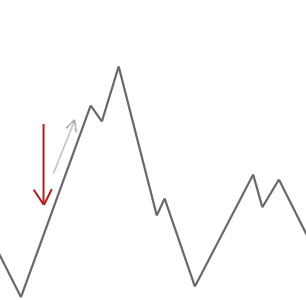
In the example above we start our hill climber off at the red arrow and it works its way up the hill until it reaches a point where it can’t climb any higher without first descending. In this example we can clearly see that it’s stuck in a local optimum. If this were a real world problem we wouldn’t know how the search space looks so unfortunately we wouldn’t be able to tell whether this solution is anywhere close to a global optimum.
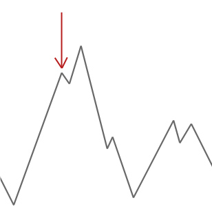
Simulated annealing works slightly differently than this and will occasionally accept worse solutions. This characteristic of simulated annealing helps it to jump out of any local optimums it might have otherwise got stuck in.
Acceptance Function
Let’s take a look at how the algorithm decides which solutions to accept so we can better understand how its able to avoid these local optimums.First we check if the neighbour solution is better than our current solution. If it is, we accept it unconditionally. If however, the neighbour solution isn’t better we need to consider a couple of factors. Firstly, how much worse the neighbour solution is; and secondly, how high the current ‘temperature’ of our system is. At high temperatures the system is more likely accept solutions that are worse.
The math for this is pretty simple:
exp( (solutionEnergy - neighbourEnergy) / temperature )
Basically, the smaller the change in energy (the quality of the solution), and the higher the temperature, the more likely it is for the algorithm to accept the solution.
Algorithm Overview
So how does the algorithm look? Well, in its most basic implementation it’s pretty simple.- First we need set the initial temperature and create a random initial solution.
- Then we begin looping until our stop condition is met. Usually either the system has sufficiently cooled, or a good-enough solution has been found.
- From here we select a neighbour by making a small change to our current solution.
- We then decide whether to move to that neighbour solution.
- Finally, we decrease the temperature and continue looping
Temperature Initialisation
For better optimisation, when initialising the temperature variable we should select a temperature that will initially allow for practically any move against the current solution. This gives the algorithm the ability to better explore the entire search space before cooling and settling in a more focused region.Example Code
Now let’s use what we know to create a basic simulated annealing algorithm, and then apply it to the traveling salesman problem below. We’re going to use Java in this tutorial, but the logic should hopefully be simple enough to copy to any language of your choice.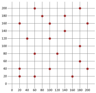
First we need to create a City class that can be used to model the different destinations of our traveling salesman.
City.java
/*
* City.java
* Models a city
*/
package sa;
public class City {
int x;
int y;
// Constructs a randomly placed city
public City(){
this.x = (int)(Math.random()*200);
this.y = (int)(Math.random()*200);
}
// Constructs a city at chosen x, y location
public City(int x, int y){
this.x = x;
this.y = y;
}
// Gets city's x coordinate
public int getX(){
return this.x;
}
// Gets city's y coordinate
public int getY(){
return this.y;
}
// Gets the distance to given city
public double distanceTo(City city){
int xDistance = Math.abs(getX() - city.getX());
int yDistance = Math.abs(getY() - city.getY());
double distance = Math.sqrt( (xDistance*xDistance) + (yDistance*yDistance) );
return distance;
}
@Override
public String toString(){
return getX()+", "+getY();
}
}
Next let’s create a class that can keep track of the cities.
TourManager.java
/*
* TourManager.java
* Holds the cities of a tour
*/
package sa;
import java.util.ArrayList;
public class TourManager {
// Holds our cities
private static ArrayList destinationCities = new ArrayList<City>();
// Adds a destination city
public static void addCity(City city) {
destinationCities.add(city);
}
// Get a city
public static City getCity(int index){
return (City)destinationCities.get(index);
}
// Get the number of destination cities
public static int numberOfCities(){
return destinationCities.size();
}
}
Now to create the class that can model a traveling salesman tour.
Tour.java
/*
* Tour.java
* Stores a candidate tour through all cities
*/
package sa;
import java.util.ArrayList;
import java.util.Collections;
public class Tour{
// Holds our tour of cities
private ArrayList tour = new ArrayList<City>();
// Cache
private int distance = 0;
// Constructs a blank tour
public Tour(){
for (int i = 0; i < TourManager.numberOfCities(); i++) {
tour.add(null);
}
}
// Constructs a tour from another tour
public Tour(ArrayList tour){
this.tour = (ArrayList) tour.clone();
}
// Returns tour information
public ArrayList getTour(){
return tour;
}
// Creates a random individual
public void generateIndividual() {
// Loop through all our destination cities and add them to our tour
for (int cityIndex = 0; cityIndex < TourManager.numberOfCities(); cityIndex++) {
setCity(cityIndex, TourManager.getCity(cityIndex));
}
// Randomly reorder the tour
Collections.shuffle(tour);
}
// Gets a city from the tour
public City getCity(int tourPosition) {
return (City)tour.get(tourPosition);
}
// Sets a city in a certain position within a tour
public void setCity(int tourPosition, City city) {
tour.set(tourPosition, city);
// If the tours been altered we need to reset the fitness and distance
distance = 0;
}
// Gets the total distance of the tour
public int getDistance(){
if (distance == 0) {
int tourDistance = 0;
// Loop through our tour's cities
for (int cityIndex=0; cityIndex < tourSize(); cityIndex++) {
// Get city we're traveling from
City fromCity = getCity(cityIndex);
// City we're traveling to
City destinationCity;
// Check we're not on our tour's last city, if we are set our
// tour's final destination city to our starting city
if(cityIndex+1 < tourSize()){
destinationCity = getCity(cityIndex+1);
}
else{
destinationCity = getCity(0);
}
// Get the distance between the two cities
tourDistance += fromCity.distanceTo(destinationCity);
}
distance = tourDistance;
}
return distance;
}
// Get number of cities on our tour
public int tourSize() {
return tour.size();
}
@Override
public String toString() {
String geneString = "|";
for (int i = 0; i < tourSize(); i++) {
geneString += getCity(i)+"|";
}
return geneString;
}
}
Finally, let’s create our simulated annealing algorithm.
SimulatedAnnealing.java
package sa;
public class SimulatedAnnealing {
// Calculate the acceptance probability
public static double acceptanceProbability(int energy, int newEnergy, double temperature) {
// If the new solution is better, accept it
if (newEnergy < energy) {
return 1.0;
}
// If the new solution is worse, calculate an acceptance probability
return Math.exp((energy - newEnergy) / temperature);
}
public static void main(String[] args) {
// Create and add our cities
City city = new City(60, 200);
TourManager.addCity(city);
City city2 = new City(180, 200);
TourManager.addCity(city2);
City city3 = new City(80, 180);
TourManager.addCity(city3);
City city4 = new City(140, 180);
TourManager.addCity(city4);
City city5 = new City(20, 160);
TourManager.addCity(city5);
City city6 = new City(100, 160);
TourManager.addCity(city6);
City city7 = new City(200, 160);
TourManager.addCity(city7);
City city8 = new City(140, 140);
TourManager.addCity(city8);
City city9 = new City(40, 120);
TourManager.addCity(city9);
City city10 = new City(100, 120);
TourManager.addCity(city10);
City city11 = new City(180, 100);
TourManager.addCity(city11);
City city12 = new City(60, 80);
TourManager.addCity(city12);
City city13 = new City(120, 80);
TourManager.addCity(city13);
City city14 = new City(180, 60);
TourManager.addCity(city14);
City city15 = new City(20, 40);
TourManager.addCity(city15);
City city16 = new City(100, 40);
TourManager.addCity(city16);
City city17 = new City(200, 40);
TourManager.addCity(city17);
City city18 = new City(20, 20);
TourManager.addCity(city18);
City city19 = new City(60, 20);
TourManager.addCity(city19);
City city20 = new City(160, 20);
TourManager.addCity(city20);
// Set initial temp
double temp = 10000;
// Cooling rate
double coolingRate = 0.003;
// Initialize intial solution
Tour currentSolution = new Tour();
currentSolution.generateIndividual();
System.out.println("Initial solution distance: " + currentSolution.getDistance());
// Set as current best
Tour best = new Tour(currentSolution.getTour());
// Loop until system has cooled
while (temp > 1) {
// Create new neighbour tour
Tour newSolution = new Tour(currentSolution.getTour());
// Get a random positions in the tour
int tourPos1 = (int) (newSolution.tourSize() * Math.random());
int tourPos2 = (int) (newSolution.tourSize() * Math.random());
// Get the cities at selected positions in the tour
City citySwap1 = newSolution.getCity(tourPos1);
City citySwap2 = newSolution.getCity(tourPos2);
// Swap them
newSolution.setCity(tourPos2, citySwap1);
newSolution.setCity(tourPos1, citySwap2);
// Get energy of solutions
int currentEnergy = currentSolution.getDistance();
int neighbourEnergy = newSolution.getDistance();
// Decide if we should accept the neighbour
if (acceptanceProbability(currentEnergy, neighbourEnergy, temp) > Math.random()) {
currentSolution = new Tour(newSolution.getTour());
}
// Keep track of the best solution found
if (currentSolution.getDistance() < best.getDistance()) {
best = new Tour(currentSolution.getTour());
}
// Cool system
temp *= 1-coolingRate;
}
System.out.println("Final solution distance: " + best.getDistance());
System.out.println("Tour: " + best);
}
}
Output
Initial solution distance: 1966
Final solution distance: 911
Tour: |180, 200|200, 160|140, 140|180, 100|180, 60|200, 40|160, 20|120, 80|100, 40|60, 20|20, 20|20, 40|60, 80|100, 120|40, 120|20, 160|60, 200|80, 180|100, 160|140, 180|
Final solution distance: 911
Tour: |180, 200|200, 160|140, 140|180, 100|180, 60|200, 40|160, 20|120, 80|100, 40|60, 20|20, 20|20, 40|60, 80|100, 120|40, 120|20, 160|60, 200|80, 180|100, 160|140, 180|
Conclusion
In this example we were able to more than half the distance of our initial randomly generated route. This hopefully goes to show how handy this relatively simple algorithm is when applied to certain types of optimisation problems.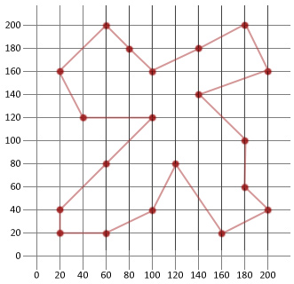
Author
 Hello, I'm Lee.
I'm a developer from the UK who writes about technology and startups. Here you'll find articles and tutorials about things that interest me. If you want to hire me or know more about me head over to my about me page
Social Links
Tweet
Follow


