Ant Colony Optimization For Hackers
Originally proposed in 1992 by Marco Dorigo, ant colony optimization (ACO) is an optimization technique inspired by the path finding behaviour of ants searching for food. ACO is also a subset of swarm intelligence - a problem solving technique using decentralized, collective behaviour, to derive artificial intelligence. Typical applications of ant colony optimization are combinatorial optimization problems such as the traveling salesman problem, however it can also be used to solve various scheduling and routing problems.One advantage ant colony optimization algorithms have over other optimization algorithms is their ability to adapt to dynamic environments - a feature that makes it great for applications such as network routing, where there are likely to be frequent changes to accommodate to.
Ants in Nature
To fully understand ant colony optimization, it’s important to first understand the natural behavior of ants which first inspired the algorithm.When searching for food ants follow a relatively simple set of rules. Although simple, these rules allow ants to communicate and cooperatively optimize their paths to food sources. The way ants do this is through the use of pheromone trails. Pheromone trails are what ants use to communicate to other ants that a food source has been found, and how to get to it. Then when other ants discover these pheromone trails they can decide whether they want to follow them. Depending on the strength of the pheromone trail an ant may decide to take a different path, but on average the stronger a pheromone trail is the more likely an ant will be to take it.
Over time, unless reinforced by other ants, pheromone trails will gradually evaporate. This means that pheromone trails which no longer lead to a food source will eventually stop being used, promoting ants to find new paths and new food sources.
To understand how over time this process also enables the colony to optimize their paths, consider the following example:
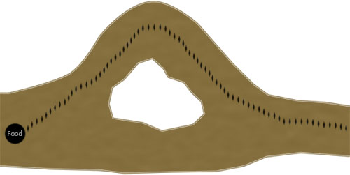
Here we can see the path an ant has taken to reach a food source. From our view of the environment we can see that although the ant may have found a valid path to the food source, it’s not the optimal one. But, here's where it get's interesting... Next, ants from the colony stumble upon the previous ant’s pheromone trail. Most take the path of the pheromone trail, but a few others decide to take the other, more direct, path:

Although the original pheromone trail may be stronger, now a second pheromone trail has started to develop from the few ants which randomly went the other way. What's important is that in this scenario the second path has an advantage because the ants taking it will reach, and retrieve the food quicker than ants following the first path. For example, using the original path it may take 3 minutes for one ant to lay a single pheromone trail from the food back to the colony, but in that time an ant may be able to lay two pheromone trails when using the shorter path. Due to this characteristic the shorter path will usually begin to acquire more pheromone than the original path over time. This then leads to the original pheromone trail being used less and eventually evaporating completely in favor of the new, shorter path.

It’s worth briefly noting here that this is only a generalization of ant behavior in nature, and that different ant species vary in their exact use of pheromones.
The Algorithm
This tutorial will look at applying the ACO algorithm to the traveling salesman problem (TSP). If you are not already familiar with the traveling salesman problem, you may want to familiarise yourself with it here, Applying a genetic algorithm to the traveling salesman problemThe bulk of the ant colony optimization algorithm is made up of only a few steps. First, each ant in the colony constructs a solution based on previously deposited pheromone trails. Next ants will lay pheromone trails on the components of their chosen solution, depending on the solution’s quality. In the example of the traveling salesman problem this would be the edges (or the paths between the cities). Finally, after all ants have finished constructing a solution and laying their pheromone trails, pheromone is evaporated from each component depending on the pheromone evaporation rate. These steps are then ran as many times as are needed to generate an adequate solution.
Constructing a Solution
As mentioned previously, an ant will often follow the strongest pheromone trail when constructing a solution. However, for the ant to consider solutions other than the current best, a small amount of randomness is required in its decision process. In addition to this, a heuristic value is also computed and considered helping to guide the search process towards the best solutions. In the example of the traveling salesman problem this heuristic will typically be the length of the edge between the city being considered - the shorter the edge, the more likely an ant will pick it.Let’s take a look at how this works mathematically:
$$p^k_{ij} = \frac{[t_{ij}]^\alpha \cdot [n_{ij}]^\beta}{\sum_{l\in N^{k}_{l}} [t_{il}]^\alpha \cdot [n_{il}]^\beta}$$
This equation calculates the probability of selecting a single component of the solution. Here, $t_{ij}$ denotes the amount of pheromone on a component between states $i$ and $j$, and $n_{ij}$ denotes it’s heuristic value. $\alpha$ and $\beta$ are both parameters used to control the importance of the pheromone trail and heuristic information during component selection.
In code this would typically be written as a roulette-wheel-style selection process:
rouletteWheel = 0
states = ant.getUnvisitedStates()
for newState in states do
rouletteWheel += Math.pow(getPheromone(state, newState), getParam('alpha'))
* Math.pow(calcHeuristicValue(state, newState), getParam('beta'))
end for
randomValue = random()
wheelPosition = 0
for newState in states do
wheelPosition += Math.pow(getPheromone(state, newState), getParam('alpha'))
* Math.pow(calcHeuristicValue(state, newState), getParam('beta'))
if wheelPosition >= randomValue do
return newState
end for
For the traveling salesman problem a state would represent a single city on the graph. Here, an ant would be selecting the next city depending on the distance to the next city, and the amount of pheromone on the path between the two cities.
Local Pheromone Update
The local pheromone update process is applied every time an ant successfully constructs a solution. This step mimics the way ants lay pheromone trails after finding food in nature. As you may remember from earlier, in nature better paths acquire more pheromone due to ants being able to traverse them quicker. In ACO, this characteristic is replicated by varying the amount of pheromone deposited on a component by considering how well the completed solution scores. If we use the traveling salesman problem as an example, pheromone will be deposited on the paths an ant took between cities depending the total tour distance.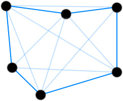
This image shows pheromone trails laid on the paths between cities in a typical traveling salesman problem.
Before looking at how it could be written in code, first let’s look at it mathematically:
$$\Delta \tau^k_{ij} = \begin{cases}Q/C^k& \text{if component(i, j) was used by ant}\\0& \text{Otherwise}\\ \end{cases}$$ $$\tau_{ij} \leftarrow \tau_{ij} + \sum_{k=1}^m \Delta \tau^k_{ij}$$
Here, $C^k$ is defined as the total cost of the solution, in the example of the traveling salesman problem this would be the tour length. $Q$ is simply a parameter to adjust the amount of pheromone deposited, typically it would be set to 1. We sum $Q/C^k$ for every solution which used $\text{component(i, j)}$, then that value becomes the amount of pheromone to be deposited on $\text{component(i, j)}$.
For clarity, let’s go over a quick example of this process when applied to the traveling salesman problem…
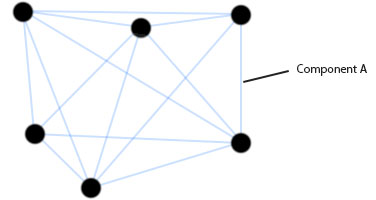
Here, we have a typical traveling salesman graph and we are interested in calculating how much pheromone should be deposited on component A. In this example, let’s assume three ants used this edge, or "component A", when constructing their tour. Let's also assume the three tours constructed had the following total distances:
Tour 1: 450
Tour 2: 380
Tour 1: 460
Tour 2: 380
Tour 1: 460
To work out how much pheromone should be deposited we simply sum the following:
componentNewPheromone = (Q / 450) + (Q / 380) + (Q / 460)
Now add that value to the pheromone on the component:
componentPheromone = componentPheromone + componentNewPheromone
Now, for a quick code example:
for ant in colony do
tour = ant.getTour();
pheromoneToAdd = getParam('Q') / tour.distance();
for cityIndex in tour do
if lastCity(cityIndex) do
edge = getEdge(cityIndex, 0)
else do
edge = getEdge(cityIndex, cityIndex+1)
end if
currentPheromone = edge.getPheromone();
edge.setPheromone(currentPheromone + pheromoneToAdd)
end for
end for
In this code example we are simply looping over the ant colony, fetching each of the tours and finally applying pheromone to each tour edge.
Global Pheromone Update
The global pheromone update is the stage in which pheromone is evaporated from components. It is applied after each iteration of the algorithm, when each ant has successfully constructed a tour and applied the local update rule.
The global pheromone update is defined mathematically as follows:
$$\tau_{ij} \leftarrow (1 - \rho) \cdot \tau_{ij}$$
Where $\tau_{ij}$ is the pheromone on the component between state $i$ and $j$ and $\rho$, is a parameter used to vary the level of evaporation.
In code this might look as follows:
for edge in edges
updatedPheromone = (1 - getParam('rho')) * edge.getPheromone()
edge.setPheromone(updatedPheromone)
end for
updatedPheromone = (1 - getParam('rho')) * edge.getPheromone()
edge.setPheromone(updatedPheromone)
end for
Optimization
There are many variations of ant colony optimization, two of the main ones being elitist and MaxMin. Depending on the problem it's likely these variations will preform better than the standard ant colony system we have looked at here. Luckily for us however, it's quite simple to extend our algorithm to include elitist and MaxMin.Elitist
In elitist ACO systems, either the best current, or global best ant, deposits extra pheromone during it's local pheromone update procedure. This encourages the colony to refine it's search around solutions which have a track record of being high quality. If all goes well, this should result in better search performance.The math for the elitist local pheromone update procedure is almost exactly the same as the the local update procedure which we previously studied, with one small update:
$$\Delta \tau^{bs}_{ij} = \begin{cases}Q/C^{bs}& \text{if component(i, j) belongs to an elite ant}\\0& \text{Otherwise}\\ \end{cases}$$ $$\tau_{ij} \leftarrow \tau_{ij} + \sum_{k=1}^m \Delta \tau^k_{ij} + e \Delta \tau^{bs}_{ij}$$
Where, $e$ is a parameter used to adjust the amount of extra pheromone given to the best (or "elite") solution.
MaxMin
The MaxMin algorithm is similar to the elitist ACO algorithm in that it gives preference to high ranking solutions. However, in MaxMin instead of simply giving extra weight to elite solutions, only the best current, or best global solution, is allowed to deposit a pheromone trail. Additionally, MaxMin requires pheromone trails are keep between a maximum and minimum value. The idea being that having a limited range between the amount of pheromone found on trails, premature convergence around sub-optimal solutions can be avoided.In many MaxMin implementations the best current ant is initially the ant which lays pheromone trails, then later, the algorithm switches so that the global best ant is the only ant which can lay a pheromone trail. This process helps encourage search across the entire search space initially, before eventually focusing in on the all time best, hopefully making a few final amendments.
Finally, the maximum and minimum value can either be passed in as parameters or adaptively set with code.
Example
To finish off here is an example implementation of the ACO algorithm applied to the traveling salesman problem in JavaScript. Simply click the graph to add new cities, then click the start button when you're ready to run the algorithm. Feel free to play around with the parameters so you get a feel for how the search process works. I've made the code available below - but please beware that I haven't finished refactoring or commenting it just yet.| Debug Info | |
| Configuration | |
| ACO Mode: | |
| Max Pheromone: | (1 * Pheromone Deposit Weight) / Best distance |
| Min Pheromone: | Max Pheromone * Scaling Factor |
| Min Scaling Factor: |
|
| Colony Size: | |
| Max Iterations: | |
| Alpha: | |
| Beta: | |
| Rho: | |
| Initial Pheromone: | |
| Pheromone Deposit Weight: | |
Download Source
Author
 Hello, I'm Lee.
I'm a developer from the UK who writes about technology and startups. Here you'll find articles and tutorials about things that interest me. If you want to hire me or know more about me head over to my about me page
Social Links
Tweet
Follow


